14 Introduction to phylogenies in R
There are lots of packages for phylogenetic analyses in R. I won’t enumerate them all here, but you can have a good idea of the options available by looking at the phylogenetic R vignette maintainned by Brian O’Meara. It is mostly oriented towards phylogenetic comparative methods, but it is a good start.
The most basic package for using trees in R is ape, which allows you to read and plot trees.
14.1 Importing and plotting trees
14.1.1 Simulate a tree
Throughout these exercises, we will often use simulated trees, which are very useful for pedagogical purposes. Trees can be simulated using several functions, but here is an example to simulate one tree with 15 species.

You save the tree in nexus format to a file. But before you do so, it is a good idea to set the working directory to the same folder where your script is saved. You can do that in RStudio in the menu Session>Set Working Directory>To Source File Location.
14.1.2 Simulating characters
Characters can also be easily simulated in R. For instance, you could simulate a character using a Brownian Motion (BM) model using the following code.
trait1 <- fastBM(tree, sig2=0.01, nsim=1, internal=FALSE)
# To get trait values for tree tips:
trait1
## t3 t4 t7 t8 t2 t14
## -0.007306853 0.043251831 0.004858391 -0.114795593 -0.043737891 0.113964926
## t15 t9 t12 t13 t5 t6
## 0.097243984 0.096978766 0.063069656 0.053040643 0.072476832 0.034675083
## t1 t10 t11
## -0.084659118 0.118596501 0.059071786Now, let’s save this trait to a file to pretend it is our original data.
write.table(matrix(trait1,ncol=1,dimnames=list(names(trait1),"trait1")), file="mytrait.csv", sep=";")Now that we have simulated a tree and a character, let’s erase what we have done so far from the R environment and pretend these are our data for the next sections.
14.2 Import data into R
Here is how you should import your data into R.
The tree format in ape contains several information and it is useful to know how to access them. For instance, the tip labels can be accessed using tree$tip.label and the branch lengths using tree$edge.length. Will will see more options in other exercises, but if you want more detailed information on how the objects “phylo” are organized, you can have a look the help file ?read.tree or at this document prepared by Emmanuel Paradis, the author of ape.
14.3 Plot trees
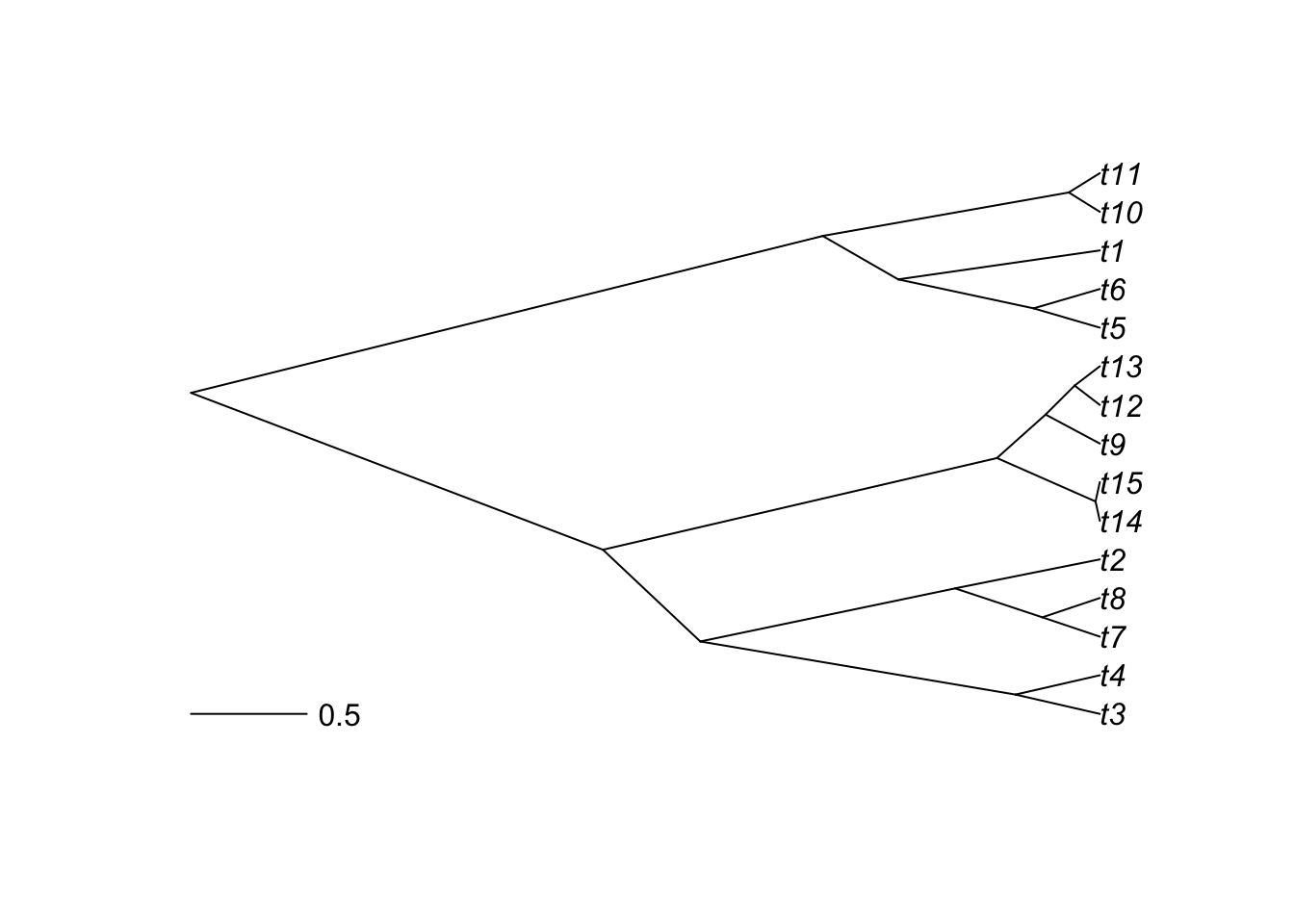
Plotting trees is one of the very interesting aspects of using R. Options are numerous and possibilities large. The most common function is plot.phylo from the ape package that has a lot of different options. I strongly suggest that you take a close look at the different options of the function ?plot.phylo. Here is a basic example.
But R is also interesting to plot characters alongside trees. If you have a categorical character, you could use it to color the tips of the phylogeny.
# Generate a random categorical character
trait2 <- as.factor(sample(c(1,2,3),size=length(tree$tip.label),replace=TRUE))
# Create color palette
library(RColorBrewer)
ColorPalette1 <- brewer.pal(n = length(levels(trait2)), name = "Dark2")
plot(tree, type="p", use.edge.length = TRUE, label.offset=0.2,cex=1)
tiplabels(pch=21,bg=ColorPalette1[trait2],col="black",cex=1,adj=0.6)
op<-par(xpd=TRUE)
legend(0,0,legend=levels(trait2),col=ColorPalette1,
       pch=20,bty="n",cex=1,pt.cex=1.5,ncol=length(levels(trait2)))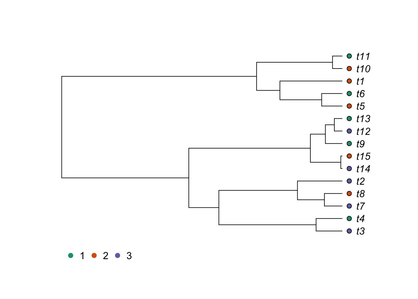
A similar result could be obtained with a continuous variable. Here, we will use the Brownian Motion model, which we will study in a further class, to simulate the continuous character.
# Breakdown continuous trait in categories
trait1.cat <- cut(trait1[,1],breaks=8,labels=FALSE)
# Create color palette
ColorPalette2 <- brewer.pal(n = 8, name = "Blues")
# Plot the tree
plot(tree, type="p", use.edge.length = TRUE, label.offset=0.2,cex=1)
tiplabels(pch=21,bg=ColorPalette2[trait1.cat],col="black",cex=1,adj=0.6)
op<-par(xpd=TRUE)
legend(0,0,legend=levels(cut(trait1[,1],breaks=8)),
       col=ColorPalette2,pch=20,bty="n",cex=0.7,pt.cex=1.5,ncol=4)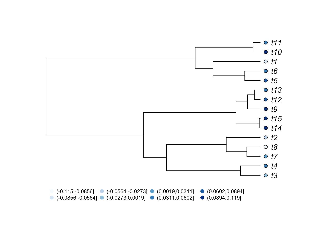
As expected from a character simlated with Brownian motion, you can see that closely related species tend to have more similar character values.
Another option to represent a continuous parameter is to use the function table.phylo4d from the adephylo package to represent the trait where its values are represented by sizes of different sizes and colors. It is also possible to plot multiple characters at the same time.
Note that you will have to install the packages phylobase and adephylo to run these function if they are not installed.
library(phylobase)
library(adephylo)
trait3 <- fastBM(tree, sig2=0.1, nsim=1, internal=FALSE) #simulate a faster evolving trait
trait.table <- data.frame(trait1=trait1[,1], trait3)
obj <- phylo4d(tree, trait.table) # build a phylo4d object
op <- par(mar=c(1,1,1,1))
table.phylo4d(obj,cex.label=1,cex.symbol=1,ratio.tree=0.8,grid=FALSE,box=FALSE)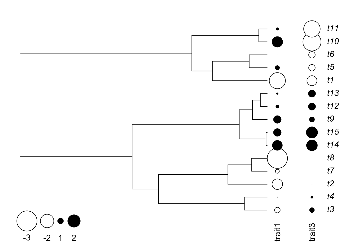
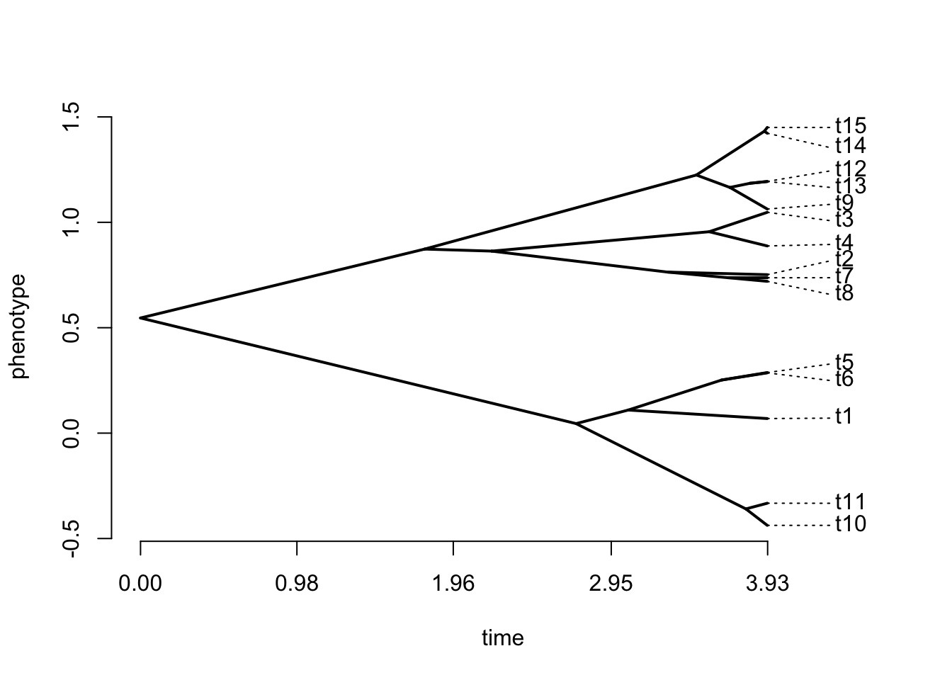
You can also represent a traitgram:
Finally, it is also possible to represent a tree on a 2-dimensional plot, coloring points with the categorical variable.
phylomorphospace(tree,trait.table)
points(trait.table,pch=21,bg=ColorPalette1[trait2],col="black",cex=1.2,adj=1)
legend("topleft",legend=levels(trait2),
       col=ColorPalette1,pch=20,bty="n",cex=1,pt.cex=1.5,ncol=length(levels(trait2)))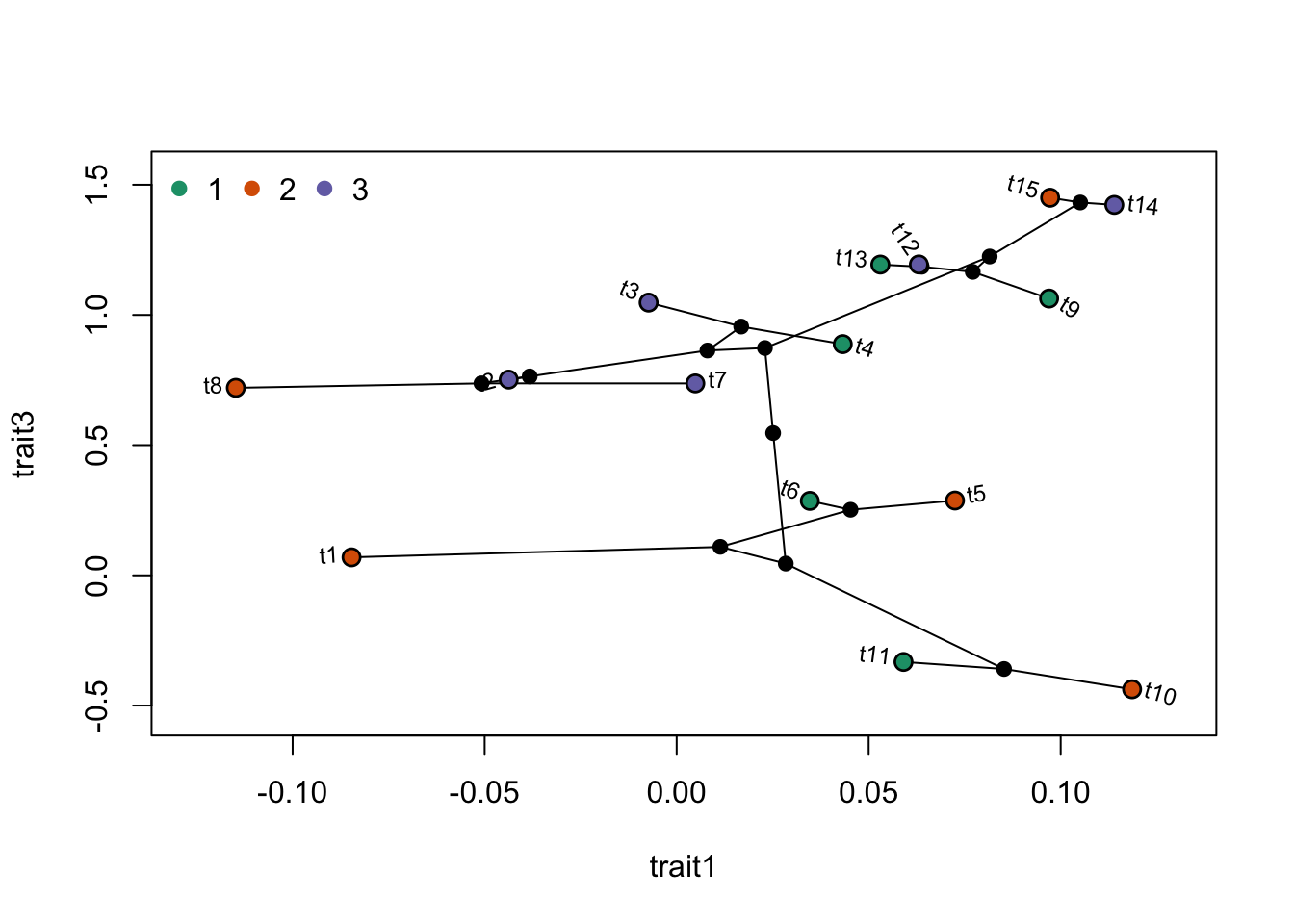
14.4 Handling multiple trees
In several cases, it is important to know how to handle multiple trees in R. These are normally stored in a multiPhylo object. Let’s see an example.
## 10 phylogenetic treesYou can see that the object is not the same as a phylo object. For instance, if you use the code plot(trees), you will be prompted to hit enter to pass from one tree to the other. To access to individual trees, you need to use the following technique.
##
## Phylogenetic tree with 15 tips and 14 internal nodes.
##
## Tip labels:
##   t3, t4, t5, t14, t15, t8, ...
##
## Rooted; includes branch lengths.
14.5 Manipulating trees
There are several manipulations that can be made to trees. Here are a few examples.

14.5.3 Get cophenetic distances
##            t3        t4        t7        t8       t2        t14        t15
## t3  0.0000000 0.7285289 3.4533793 3.4533793 3.453379 4.29496600 4.29496600
## t4  0.7285289 0.0000000 3.4533793 3.4533793 3.453379 4.29496600 4.29496600
## t7  3.4533793 3.4533793 0.0000000 0.4962115 1.250834 4.29496600 4.29496600
## t8  3.4533793 3.4533793 0.4962115 0.0000000 1.250834 4.29496600 4.29496600
## t2  3.4533793 3.4533793 1.2508336 1.2508336 0.000000 4.29496600 4.29496600
## t14 4.2949660 4.2949660 4.2949660 4.2949660 4.294966 0.00000000 0.03691962
## t15 4.2949660 4.2949660 4.2949660 4.2949660 4.294966 0.03691962 0.00000000
## t9  4.2949660 4.2949660 4.2949660 4.2949660 4.294966 0.88909442 0.88909442
## t12 4.2949660 4.2949660 4.2949660 4.2949660 4.294966 0.88909442 0.88909442
## t13 4.2949660 4.2949660 4.2949660 4.2949660 4.294966 0.88909442 0.88909442
## t5  7.8556290 7.8556290 7.8556290 7.8556290 7.855629 7.85562897 7.85562897
## t6  7.8556290 7.8556290 7.8556290 7.8556290 7.855629 7.85562897 7.85562897
## t1  7.8556290 7.8556290 7.8556290 7.8556290 7.855629 7.85562897 7.85562897
## t10 7.8556290 7.8556290 7.8556290 7.8556290 7.855629 7.85562897 7.85562897
## t11 7.8556290 7.8556290 7.8556290 7.8556290 7.855629 7.85562897 7.85562897
##            t9       t12       t13        t5        t6       t1      t10
## t3  4.2949660 4.2949660 4.2949660 7.8556290 7.8556290 7.855629 7.855629
## t4  4.2949660 4.2949660 4.2949660 7.8556290 7.8556290 7.855629 7.855629
## t7  4.2949660 4.2949660 4.2949660 7.8556290 7.8556290 7.855629 7.855629
## t8  4.2949660 4.2949660 4.2949660 7.8556290 7.8556290 7.855629 7.855629
## t2  4.2949660 4.2949660 4.2949660 7.8556290 7.8556290 7.855629 7.855629
## t14 0.8890944 0.8890944 0.8890944 7.8556290 7.8556290 7.855629 7.855629
## t15 0.8890944 0.8890944 0.8890944 7.8556290 7.8556290 7.855629 7.855629
## t9  0.0000000 0.4685481 0.4685481 7.8556290 7.8556290 7.855629 7.855629
## t12 0.4685481 0.0000000 0.2174902 7.8556290 7.8556290 7.855629 7.855629
## t13 0.4685481 0.2174902 0.0000000 7.8556290 7.8556290 7.855629 7.855629
## t5  7.8556290 7.8556290 7.8556290 0.0000000 0.5720997 1.742611 2.395633
## t6  7.8556290 7.8556290 7.8556290 0.5720997 0.0000000 1.742611 2.395633
## t1  7.8556290 7.8556290 7.8556290 1.7426110 1.7426110 0.000000 2.395633
## t10 7.8556290 7.8556290 7.8556290 2.3956328 2.3956328 2.395633 0.000000
## t11 7.8556290 7.8556290 7.8556290 2.3956328 2.3956328 2.395633 0.268201
##          t11
## t3  7.855629
## t4  7.855629
## t7  7.855629
## t8  7.855629
## t2  7.855629
## t14 7.855629
## t15 7.855629
## t9  7.855629
## t12 7.855629
## t13 7.855629
## t5  2.395633
## t6  2.395633
## t1  2.395633
## t10 0.268201
## t11 0.000000