15 Solutions to the challenges
15.1 Challenge 1
In the seedplantsdata data frame, there were many different traits. Try to fit a regression of tree shade tolerance (shade) on the seed mass (Sm). In other words, test if shade tolerance can be explained by the seed mass of the trees. Then, try to see if the residuals are phylogenetically correlated.
# Fit a linear model using Ordinary Least Squares (OLS)
Sm.lm <- lm(Shade ~ Sm, data = seedplantsdata)
# Get the results
summary(Sm.lm)
##
## Call:
## lm(formula = Shade ~ Sm, data = seedplantsdata)
##
## Residuals:
## Min 1Q Median 3Q Max
## -1.9042 -0.9009 0.1481 0.5982 2.0962
##
## Coefficients:
## Estimate Std. Error t value Pr(>|t|)
## (Intercept) 2.904e+00 1.608e-01 18.064 <2e-16 ***
## Sm -5.824e-05 5.640e-05 -1.033 0.306
## ---
## Signif. codes: 0 '***' 0.001 '**' 0.01 '*' 0.05 '.' 0.1 ' ' 1
##
## Residual standard error: 1.149 on 55 degrees of freedom
## Multiple R-squared: 0.01902, Adjusted R-squared: 0.001184
## F-statistic: 1.066 on 1 and 55 DF, p-value: 0.3063# Extract the residuals
Sm.res <- residuals(Sm.lm)
# Plot the residuals beside the phylogeny
op <- par(mar=c(1,1,1,1))
plot(seedplantstree,type="p",TRUE,label.offset=0.01,cex=0.5,no.margin=FALSE)
tiplabels(pch=21,bg=cols[ifelse(Sm.res>0,1,2)],col="black",cex=abs(Sm.res),adj=0.505)
legend("topleft",legend=c("-2","-1","0","1","2"),pch=21,
pt.bg=cols[c(1,1,1,2,2)],bty="n",
text.col="gray32",cex=0.8,pt.cex=c(2,1,0.1,1,2))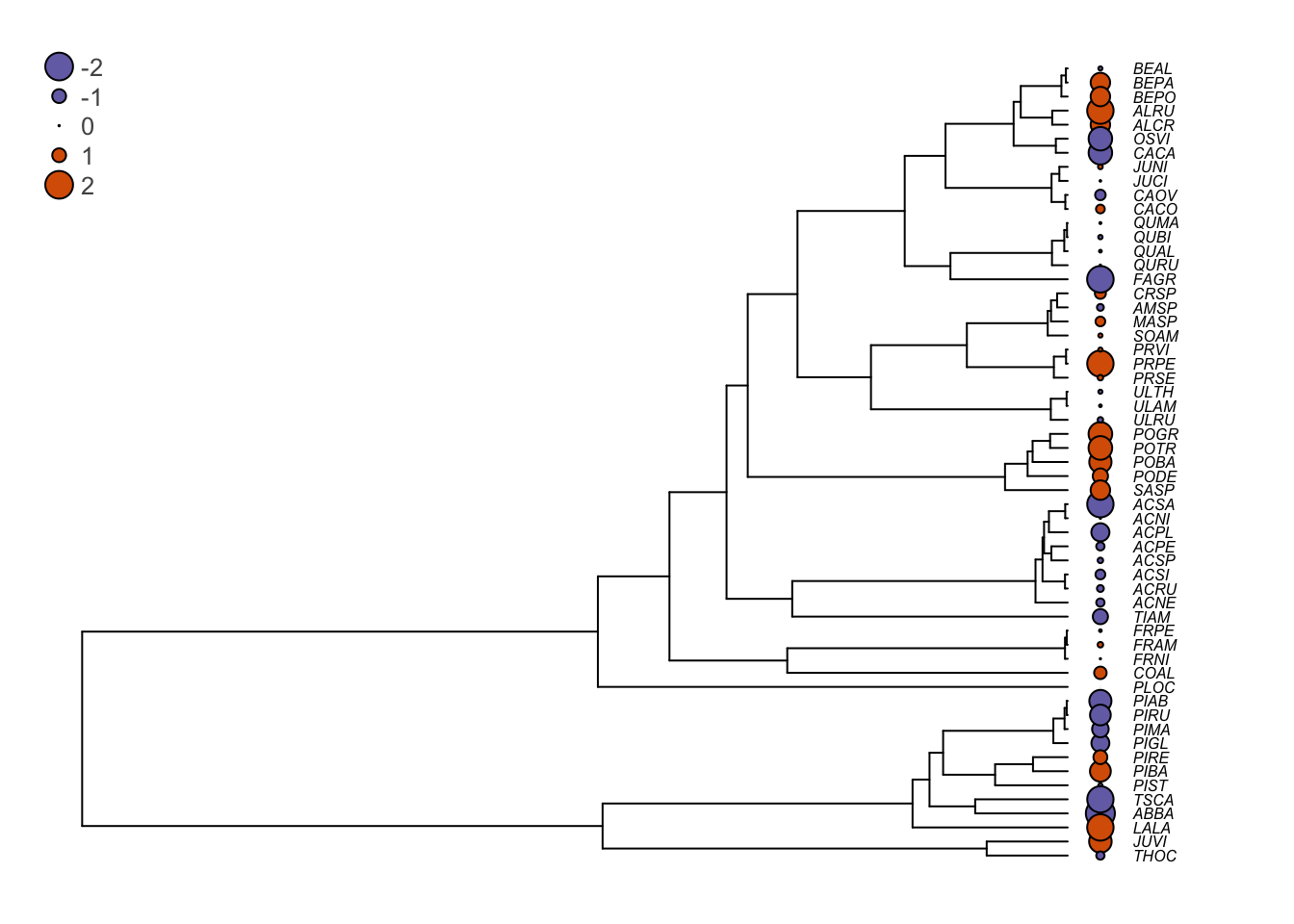
15.2 Challenge 2
Can you get the covariance matrix and the correlation matrix for the seed plants phylogenetic tree from the example above (seedplantstree)?
# Covariance matrix
seedplants.cov <- vcv(seedplantstree,corr=FALSE)
# Check the first few lines of the matrix
head(round(seedplants.cov,3))
## ABBA ACNE ACNI ACPE ACPL ACRU ACSA ACSI ACSP ALCR ALRU AMSP
## ABBA 0.151 0.000 0.000 0.000 0.000 0.000 0.000 0.000 0.000 0.000 0.000 0.000
## ACNE 0.000 0.151 0.146 0.146 0.146 0.146 0.146 0.146 0.146 0.099 0.099 0.099
## ACNI 0.000 0.146 0.151 0.147 0.148 0.147 0.150 0.147 0.147 0.099 0.099 0.099
## ACPE 0.000 0.146 0.147 0.151 0.147 0.147 0.147 0.147 0.148 0.099 0.099 0.099
## ACPL 0.000 0.146 0.148 0.147 0.151 0.147 0.148 0.147 0.147 0.099 0.099 0.099
## ACRU 0.000 0.146 0.147 0.147 0.147 0.151 0.147 0.150 0.147 0.099 0.099 0.099
## BEAL BEPA BEPO CACA CACO CAOV COAL CRSP FAGR FRAM FRNI FRPE JUCI
## ABBA 0.000 0.000 0.000 0.000 0.000 0.000 0.00 0.000 0.000 0.00 0.00 0.00 0.000
## ACNE 0.099 0.099 0.099 0.099 0.099 0.099 0.09 0.099 0.099 0.09 0.09 0.09 0.099
## ACNI 0.099 0.099 0.099 0.099 0.099 0.099 0.09 0.099 0.099 0.09 0.09 0.09 0.099
## ACPE 0.099 0.099 0.099 0.099 0.099 0.099 0.09 0.099 0.099 0.09 0.09 0.09 0.099
## ACPL 0.099 0.099 0.099 0.099 0.099 0.099 0.09 0.099 0.099 0.09 0.09 0.09 0.099
## ACRU 0.099 0.099 0.099 0.099 0.099 0.099 0.09 0.099 0.099 0.09 0.09 0.09 0.099
## JUNI JUVI LALA MASP OSVI PIAB PIBA PIGL PIMA PIRE PIRU PIST PLOC
## ABBA 0.000 0.08 0.127 0.000 0.000 0.13 0.13 0.13 0.13 0.13 0.13 0.13 0.000
## ACNE 0.099 0.00 0.000 0.099 0.099 0.00 0.00 0.00 0.00 0.00 0.00 0.00 0.079
## ACNI 0.099 0.00 0.000 0.099 0.099 0.00 0.00 0.00 0.00 0.00 0.00 0.00 0.079
## ACPE 0.099 0.00 0.000 0.099 0.099 0.00 0.00 0.00 0.00 0.00 0.00 0.00 0.079
## ACPL 0.099 0.00 0.000 0.099 0.099 0.00 0.00 0.00 0.00 0.00 0.00 0.00 0.079
## ACRU 0.099 0.00 0.000 0.099 0.099 0.00 0.00 0.00 0.00 0.00 0.00 0.00 0.079
## POBA PODE POGR POTR PRPE PRSE PRVI QUAL QUBI QUMA QURU SASP
## ABBA 0.000 0.000 0.000 0.000 0.000 0.000 0.000 0.000 0.000 0.000 0.000 0.000
## ACNE 0.099 0.099 0.099 0.099 0.099 0.099 0.099 0.099 0.099 0.099 0.099 0.099
## ACNI 0.099 0.099 0.099 0.099 0.099 0.099 0.099 0.099 0.099 0.099 0.099 0.099
## ACPE 0.099 0.099 0.099 0.099 0.099 0.099 0.099 0.099 0.099 0.099 0.099 0.099
## ACPL 0.099 0.099 0.099 0.099 0.099 0.099 0.099 0.099 0.099 0.099 0.099 0.099
## ACRU 0.099 0.099 0.099 0.099 0.099 0.099 0.099 0.099 0.099 0.099 0.099 0.099
## SOAM THOC TIAM TSCA ULAM ULRU ULTH
## ABBA 0.000 0.08 0.000 0.137 0.000 0.000 0.000
## ACNE 0.099 0.00 0.109 0.000 0.099 0.099 0.099
## ACNI 0.099 0.00 0.109 0.000 0.099 0.099 0.099
## ACPE 0.099 0.00 0.109 0.000 0.099 0.099 0.099
## ACPL 0.099 0.00 0.109 0.000 0.099 0.099 0.099
## ACRU 0.099 0.00 0.109 0.000 0.099 0.099 0.099# Correlation matrix
seedplants.cor <- vcv(seedplantstree,corr=TRUE)
# Check the first few lines of the matrix
head(round(seedplants.cor,3))## ABBA ACNE ACNI ACPE ACPL ACRU ACSA ACSI ACSP ALCR ALRU AMSP
## ABBA 1 0.000 0.000 0.000 0.000 0.000 0.000 0.000 0.000 0.000 0.000 0.000
## ACNE 0 1.000 0.967 0.967 0.967 0.967 0.967 0.967 0.967 0.654 0.654 0.654
## ACNI 0 0.967 1.000 0.976 0.981 0.974 0.997 0.974 0.976 0.654 0.654 0.654
## ACPE 0 0.967 0.976 1.000 0.976 0.974 0.976 0.974 0.983 0.654 0.654 0.654
## ACPL 0 0.967 0.981 0.976 1.000 0.974 0.981 0.974 0.976 0.654 0.654 0.654
## ACRU 0 0.967 0.974 0.974 0.974 1.000 0.974 0.997 0.974 0.654 0.654 0.654
## BEAL BEPA BEPO CACA CACO CAOV COAL CRSP FAGR FRAM FRNI FRPE
## ABBA 0.000 0.000 0.000 0.000 0.000 0.000 0.000 0.000 0.000 0.000 0.000 0.000
## ACNE 0.654 0.654 0.654 0.654 0.654 0.654 0.596 0.654 0.654 0.596 0.596 0.596
## ACNI 0.654 0.654 0.654 0.654 0.654 0.654 0.596 0.654 0.654 0.596 0.596 0.596
## ACPE 0.654 0.654 0.654 0.654 0.654 0.654 0.596 0.654 0.654 0.596 0.596 0.596
## ACPL 0.654 0.654 0.654 0.654 0.654 0.654 0.596 0.654 0.654 0.596 0.596 0.596
## ACRU 0.654 0.654 0.654 0.654 0.654 0.654 0.596 0.654 0.654 0.596 0.596 0.596
## JUCI JUNI JUVI LALA MASP OSVI PIAB PIBA PIGL PIMA PIRE PIRU PIST
## ABBA 0.000 0.000 0.528 0.843 0.000 0.000 0.86 0.86 0.86 0.86 0.86 0.86 0.86
## ACNE 0.654 0.654 0.000 0.000 0.654 0.654 0.00 0.00 0.00 0.00 0.00 0.00 0.00
## ACNI 0.654 0.654 0.000 0.000 0.654 0.654 0.00 0.00 0.00 0.00 0.00 0.00 0.00
## ACPE 0.654 0.654 0.000 0.000 0.654 0.654 0.00 0.00 0.00 0.00 0.00 0.00 0.00
## ACPL 0.654 0.654 0.000 0.000 0.654 0.654 0.00 0.00 0.00 0.00 0.00 0.00 0.00
## ACRU 0.654 0.654 0.000 0.000 0.654 0.654 0.00 0.00 0.00 0.00 0.00 0.00 0.00
## PLOC POBA PODE POGR POTR PRPE PRSE PRVI QUAL QUBI QUMA QURU
## ABBA 0.000 0.000 0.000 0.000 0.000 0.000 0.000 0.000 0.000 0.000 0.000 0.000
## ACNE 0.523 0.654 0.654 0.654 0.654 0.654 0.654 0.654 0.654 0.654 0.654 0.654
## ACNI 0.523 0.654 0.654 0.654 0.654 0.654 0.654 0.654 0.654 0.654 0.654 0.654
## ACPE 0.523 0.654 0.654 0.654 0.654 0.654 0.654 0.654 0.654 0.654 0.654 0.654
## ACPL 0.523 0.654 0.654 0.654 0.654 0.654 0.654 0.654 0.654 0.654 0.654 0.654
## ACRU 0.523 0.654 0.654 0.654 0.654 0.654 0.654 0.654 0.654 0.654 0.654 0.654
## SASP SOAM THOC TIAM TSCA ULAM ULRU ULTH
## ABBA 0.000 0.000 0.528 0.00 0.906 0.000 0.000 0.000
## ACNE 0.654 0.654 0.000 0.72 0.000 0.654 0.654 0.654
## ACNI 0.654 0.654 0.000 0.72 0.000 0.654 0.654 0.654
## ACPE 0.654 0.654 0.000 0.72 0.000 0.654 0.654 0.654
## ACPL 0.654 0.654 0.000 0.72 0.000 0.654 0.654 0.654
## ACRU 0.654 0.654 0.000 0.72 0.000 0.654 0.654 0.65415.3 Challenge 3
Fit a PGLS model to see whether the seed mass (Sm) explains shade tolerance (Shade) with the seedplantdataset. How does it compare to the results from the standard regression.
# Fit a PGLS with the gls function
Sm.pgls <- gls(Shade ~ Sm, data = seedplantsdata, correlation=bm.corr)
# Get the results
summary(Sm.pgls)
## Generalized least squares fit by REML
## Model: Shade ~ Sm
## Data: seedplantsdata
## AIC BIC logLik
## 240.3701 246.3921 -117.1851
##
## Correlation Structure: corBrownian
## Formula: ~Code
## Parameter estimate(s):
## numeric(0)
##
## Coefficients:
## Value Std.Error t-value p-value
## (Intercept) 2.8031105 4.591805 0.6104594 0.5441
## Sm -0.0000417 0.000081 -0.5117076 0.6109
##
## Correlation:
## (Intr)
## Sm -0.004
##
## Standardized residuals:
## Min Q1 Med Q3 Max
## -0.22901901 -0.10170487 0.02535202 0.08873220 0.27907713
##
## Residual standard error: 7.873115
## Degrees of freedom: 57 total; 55 residual# Extract the residuals corrected by the correlation structure
Sm.pgls.res <- residuals(Sm.pgls,type="normalized")
# Plot the residuals beside the phylogeny
op <- par(mar=c(1,1,1,1))
plot(seedplantstree,type="p",TRUE,label.offset=0.01,cex=0.5,no.margin=FALSE)
tiplabels(pch=21,bg=cols[ifelse(Sm.pgls.res>0,1,2)],col="black",cex=abs(Sm.pgls.res),adj=0.505)
legend("topleft",legend=c("-2","-1","0","1","2"),pch=21,
pt.bg=cols[c(1,1,1,2,2)],bty="n",
text.col="gray32",cex=0.8,pt.cex=c(2,1,0.1,1,2))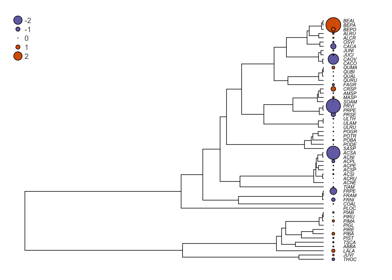
15.4 Challenge 4
Try to fit a PGLS with a Pagel correlation structure when regressing Shade tolerance on seed mass. Are the residuals as phylogenetically correlated than in the previous regression with wood density?
# Fit a PGLS with the gls function
Sm.pgls2 <- gls(Shade ~ Sm, data = seedplantsdata, correlation=pagel.corr)
# Get the results
summary(Sm.pgls2)
## Generalized least squares fit by REML
## Model: Shade ~ Sm
## Data: seedplantsdata
## AIC BIC logLik
## 187.6889 195.7183 -89.84447
##
## Correlation Structure: corPagel
## Formula: ~Code
## Parameter estimate(s):
## lambda
## 0.951553
##
## Coefficients:
## Value Std.Error t-value p-value
## (Intercept) 2.8204268 1.497276 1.883705 0.0649
## Sm -0.0000716 0.000060 -1.193604 0.2378
##
## Correlation:
## (Intr)
## Sm -0.009
##
## Standardized residuals:
## Min Q1 Med Q3 Max
## -0.6946682 -0.3115198 0.1068607 0.2604470 0.8319385
##
## Residual standard error: 2.620527
## Degrees of freedom: 57 total; 55 residual