3 An introduction to Phylogenetic Comparative Methods

Phylogenetic comparative methods were introduced by Joseph Felsenstein in 1985. The idea of phylogenetic comparative methods was to correct for the non-independence of species in statistical tests because of their shared evolutionary histories. Indeed, two species may look similar not because they live in the same environment but because they are closely related. Consider the following angiosperm phylogeny.

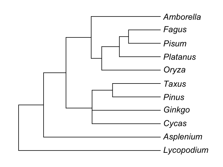
Figure 3.1: land plant phylogeny

It is clear that Fagus (beech) and Pisum (pea) are more likely to share similar characteristics compared to Asplenium (a fern), because they share a more recent common ancestor. In other words, their evolutionary histories are shared over a longer period than with Asplenium. As such, they have more chance to have more similar traits (and in fact they do). For instance, take two characters, ovule and fertilization type, within this group.

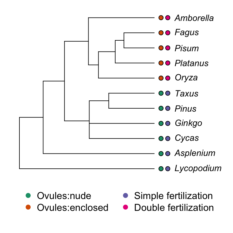
Ignoring the phylogeny, we might be tempted to see a strong correlation between these two characters. Indeed, the states between the two characters show a perfect correspondence. Using standard contingency table statistics, we could do a Fisher exact test:

fisher.test(matrix(c(5,0,0,6),ncol=2))

## 
##  Fisher's Exact Test for Count Data
## 
## data:  matrix(c(5, 0, 0, 6), ncol = 2)
## p-value = 0.002165
## alternative hypothesis: true odds ratio is not equal to 1
## 95 percent confidence interval:
##  2.842809      Inf
## sample estimates:
## odds ratio 
##        Inf

The test suggests that the assotiation is highly significant. However, we know that the comparisons made are not completely independent. Actually, both characters evolved only once, and this along the same branch.

A more appropriate way to frame the question would be “what is the probability that two characters evolved along the same branch?”. This can also be calculated using a contingency table, but this time taking the branches of the phylogeny as the units of observation.

In the example, there are 18 branches and the two characters evolved only once and on the same branch. The contingency table when considering the changes along the branches looks like this:

	Change in trait 2	No change in trait 2
Change in trait 1	1	0
No change in trait 1	0	17

With this table, Fisher’s exact test will give the following result:

fisher.test(matrix(c(1,0,0,17),ncol=2))

## 
##  Fisher's Exact Test for Count Data
## 
## data:  matrix(c(1, 0, 0, 17), ncol = 2)
## p-value = 0.05556
## alternative hypothesis: true odds ratio is not equal to 1
## 95 percent confidence interval:
##  0.4358974       Inf
## sample estimates:
## odds ratio 
##        Inf

You can see that the result is no longer significant.

While this approach for taking into account the phylogenetic relationships is correct, more powerful comparative methods have been developed. One useful and powerful approach is the Phylogenetic Generalized Least Squares (PGLS). But before we introduce PGLS, we do some revision and look briefly at the standard regression.