7 Relaxing the assumption that residuals need to be perfectly phylogenetically correlated
Phylogenetic Generalized Least Squares assume that the residuals are perfectly phylogenetically correlated. This is relatively constraining because it means that other sources of errors that are not phylogenetically correlated are not allowed by the model. Moreover, if these exist, they can bias the results of the PGLS (Revell 2010).
There are ways to relax this assumption, and one of this is to use a type of correlation structure that allows to relax this assumption.
7.1 Theory: Pagel’s correlation structure
When controling for phylogenetic relationships with phylogenetic generalized least squares, we assume that the residuals are perfectly correlated according to the correlation structure. In practice, it might not be always the case and it is difficult to really know how important it is to control for the phylogenetic relationship in a specific case. For instance, for a given study, the correlation in the residuals might not be highly phylogenetically correlated.
This is possible to account for this using the \(\lambda\) model of Pagel (Pagel 1999). The idea is to multiply the off-diagonal of the correlation matrix (essentially the branch lengths of the phylogeny) by a parameter \(\lambda\), but not the diagonal values. This essentially leads to a modification of branch lengths of the phylogeny. A \(\lambda\) value near zero gives very shorts internal branches and long tip branches. This, in effect, reduces the phylogenetic correlations (the effect of the phylogeny is reduced). At the opposite, if \(\lambda\) is close to 1, then the modified phylogeny resembles the true phylogeny. Indeed, the parameter \(\lambda\) is often interpreted as a parameter of phylogenetic signal; as such, a greater \(\lambda\) value implies a stronger phylogenetic signal.
The following figure shows how different lambda values affect the shape of the Quebec trees phylogeny.
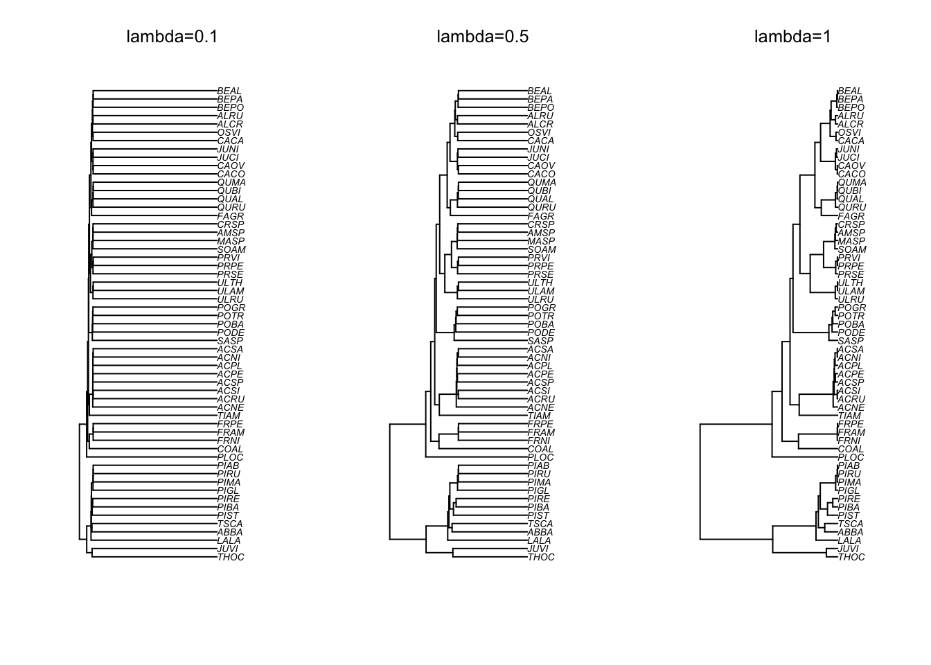
You can see that with small values of lambda, the weight given to the shared history (the phylogeny) are greatly reduced. The long terminal branches somewhat indicates that there could be a lot more variation in the residuals that are independent of the other species. This variation could be due to other factors that are included in the estimates of each species but that are independent of the phylogeny (such as measurement errors for instance).
7.2 Practicals
Pagel’s \(\lambda\) model can be used in PGLS using the corPagel correlation structure. The usage of this correlation structure is similar to that of the corBrownian structure, except that you need to provide a starting parameter value for \(\lambda\).
# Get the correlation structure
pagel.corr <- corPagel(0.3, phy=seedplantstree, fixed=FALSE, form=~Code)
The value given to corPagel is the starting value for the \(\lambda\) parameter. Also, note that the option fixed= is set to FALSE This means that the \(\lambda\) parameter will be optimized using generalized least squares. If it was set to TRUE, then the model would be fitted with the starting parameter, here 0.3. The form=~Code points to the column Code of the dataset for ordering the tree in the same order as the dataframe when fitting the function.
Let’s now fit the PGLS with this correlation structure.
# PGLS with coraPagel
shade.pgls2 <- gls(Shade ~ Wd, data = seedplantsdata, correlation=pagel.corr)
summary(shade.pgls2)
## Generalized least squares fit by REML
## Model: Shade ~ Wd
## Data: seedplantsdata
## AIC BIC logLik
## 163.3967 171.426 -77.69833
##
## Correlation Structure: corPagel
## Formula: ~Code
## Parameter estimate(s):
## lambda
## 0.9581665
##
## Coefficients:
## Value Std.Error t-value p-value
## (Intercept) 1.254987 1.636575 0.7668377 0.4465
## Wd 3.573527 1.497808 2.3858381 0.0205
##
## Correlation:
## (Intr)
## Wd -0.397
##
## Standardized residuals:
## Min Q1 Med Q3 Max
## -0.75145692 -0.44908843 -0.05417524 0.25655008 0.96493685
##
## Residual standard error: 2.621947
## Degrees of freedom: 57 total; 55 residualYou can see that gls has estimated the \(\lambda\) parameter, which is 0.958 here. Because the estimated \(\lambda\) is very close to 1, we can conclude that residuals of the model were strongly phylogenetically correlated. This, in turns, thus confirms the importance of using a PGLS with this model. If the \(\lambda\) estimated would have been close to 0, it would have suggested that the PGLS is not necessary. Note, however, that using this approach assures you to never obtained a biased statistical result. Actually, I strongly recommend that you always use this correlation structure in your statistical analyses.
7.3 Challenge 4
Try to fit a PGLS with a Pagel correlation structure when regressing Shade tolerance on seed mass. Are the residuals as phylogenetically correlated than in the previous regression with wood density?
7.4 Other correlation structures (or evolutionary models)
The correlation structures available in the package ape offer other alternatives for the assumed model of character evolution. For instance, the corMartins correlation structure models selection using the Ornstein-Uhlenbeck (or Hansen) model with parameter \(\alpha\) that determines the strength of the selection. Also, corBlomberg models accelerating or decelerating Brownian evolution, that is, the evolutionary rate of the Brownian motion is either accelerating or decelerating with time with this model. It is possible to do model comparisons to decide which model best fit the residual variation.