5 Phylogenetic generalized least squares (PGLS)
5.1 Theory
Phylogenetic generalized least squares (PGLS) is just a specific application of the broader method called generalized least squares (GLS). Generalized least squares relax the assumption that the error of the linear model has to be uncorrelated. They allow the user to specify the structure of that residual correlation. This is used, for instance, to correct for spatial correlation, time series, or phylogenetic correlation.
GLS have the same structure as Ordinary Least Squares (OLS):
\[\textbf{y} = \alpha + \beta \textbf{x} + \textbf{e}\]
The only difference is that the residuals are correlated with each other according to a correlation structure \(\textbf{C}\):
\[\textbf{e} \sim N(0,\sigma^2\textbf{C})\]
Here, \(\textbf{C}\) is a correlation matrix that describes how the residuals are correlated with each other. To be able to account for phylogenetic relationships in a PGLS, we thus need to be able to express the phylogenetic relationships in the form of a correlation matrix.
5.1.1 Phylogenetic correlation structure
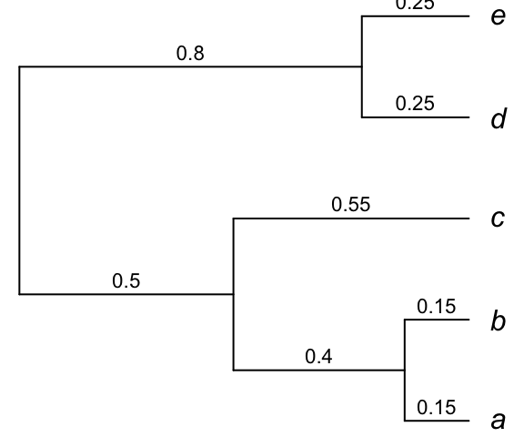
Phylogenetic relationships can be described using a correlation structure. Below, you have phylogenetic tree with branch lengths indicated above the branches.
Now, this tree can be perfectly represented by a variance-covariance matrix.
##      a    b    c    d    e
## a 1.05 0.90 0.50 0.00 0.00
## b 0.90 1.05 0.50 0.00 0.00
## c 0.50 0.50 1.05 0.00 0.00
## d 0.00 0.00 0.00 1.05 0.80
## e 0.00 0.00 0.00 0.80 1.05
The diagonal elements of the matrix are the species variances; these numbers represent the total distance from the root of the tree to the tips. It determines how much the tips have evolved from the root. The off-diagonal elements are the covariances between the species. They indicate the proportion of the time that the species have evolved together. This corresponds to the length of the branches that two species share, starting from the root of the tree. For instance, species \(a\) and \(c\) have shared a common history for 0.5 units of time; hence they have a covariance of 0.5. The greater the covariance, the longer the two species have shared the same evolutionary history.
If all the variation among species was due to phylogeny and none to selection, then this variance-covariance matrix would represent the expectation of how much all species would be similar to the other species.
Note that all the tips are equidistant from the root. When trees have this property, they are said to be ultrametric. Most phylogenetic comparative methods require the trees to be ultrametric, although there are sometimes ways to relax this assumption. If you do not have an ultrametric tree, it is possible to make it ultrametric using the function
chronoplof theapepackage. But ideally, it is better to use a phylogenetic method that directly reconstruct ultrametric trees.
The variance-covariance matrix of a phylogenetic tree can be obtained from a tree using the function vcv from the ape package.
# 'atree' corresponds to the phylogenetic tree shown above in newick format
atree <- "(((a:0.15,b:0.15):0.4,c:0.55):0.5,(d:0.25,e:0.25):0.8);"
# Let's now read this tree and store it as a phylogenetic tree object in R
atree <- read.tree(text=atree)
# Show the tree
plot(atree)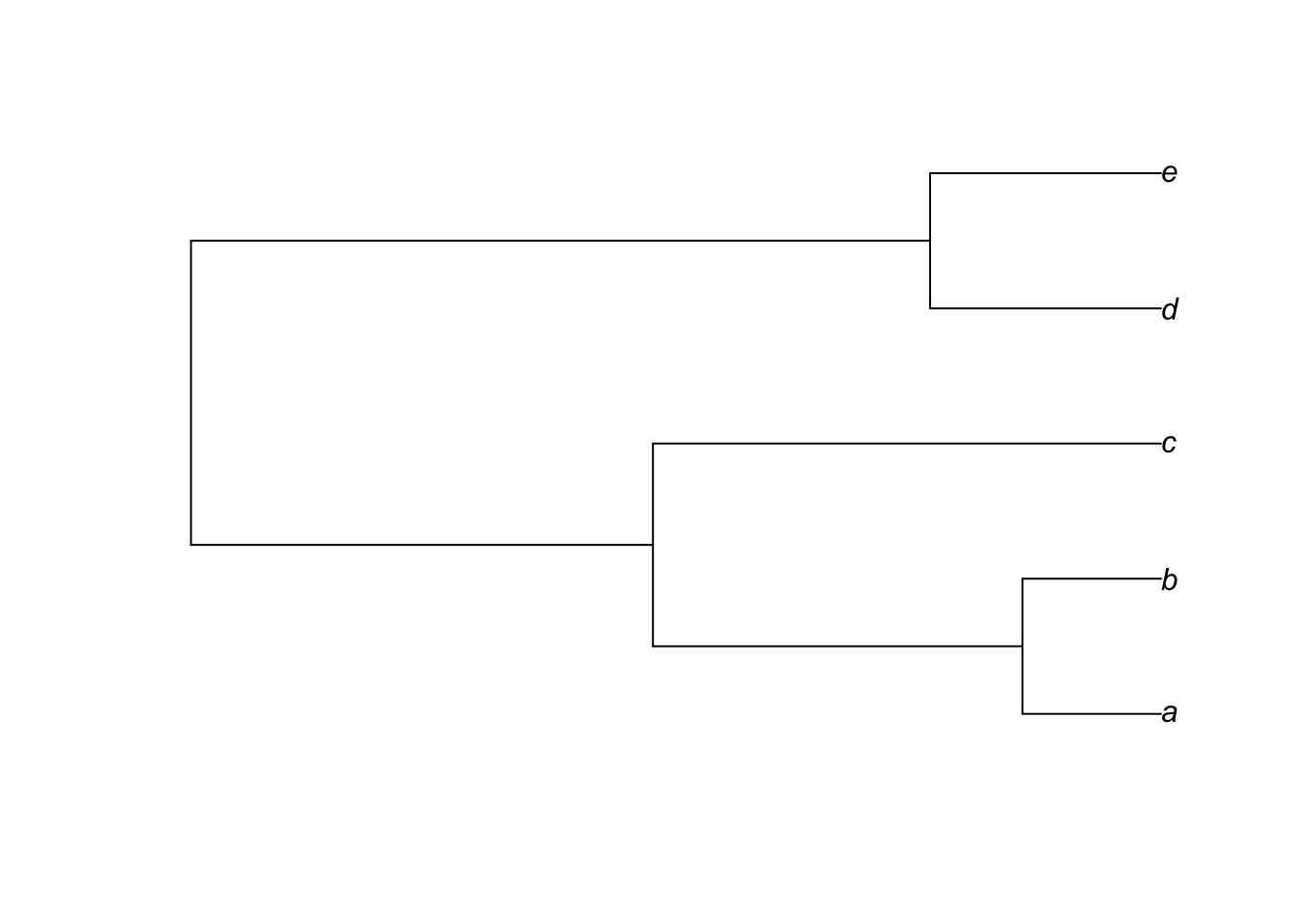
# Extract the variance-covariance matrix
varcovar <- vcv(atree)
# Print the variance-covariance matrix
varcovar
## a b c d e
## a 1.05 0.90 0.50 0.00 0.00
## b 0.90 1.05 0.50 0.00 0.00
## c 0.50 0.50 1.05 0.00 0.00
## d 0.00 0.00 0.00 1.05 0.80
## e 0.00 0.00 0.00 0.80 1.05This is great, but we mentioned above that it is a correlation matric that we need in a GLS to account for the correlation in the residuals. To obtain a correlation matrix from the variance-covariance matrix shown above, you only need to divide the variance-covariance matrix by the length of the tree, or the distance from the root to the tips. It can also be obtained using the R function cov2cor.
# Convert the covariance matrix to a correlation matrix
corrmat <- cov2cor(varcovar)
# Print the matrix, rounding the numbers to three decimals
round(corrmat,3)
## a b c d e
## a 1.000 0.857 0.476 0.000 0.000
## b 0.857 1.000 0.476 0.000 0.000
## c 0.476 0.476 1.000 0.000 0.000
## d 0.000 0.000 0.000 1.000 0.762
## e 0.000 0.000 0.000 0.762 1.000Now, the diagonal elements equal to 1, indicating that the species are perfectly correlated to themselves. Note that it is also possible to obtain directly the correlation matrix from the function vcv by using the corr=TRUE option.
# Obtaining a correlation matrix using the 'vcv' function
corrmat <- vcv(atree,corr=TRUE)
round(corrmat,3)
## a b c d e
## a 1.000 0.857 0.476 0.000 0.000
## b 0.857 1.000 0.476 0.000 0.000
## c 0.476 0.476 1.000 0.000 0.000
## d 0.000 0.000 0.000 1.000 0.762
## e 0.000 0.000 0.000 0.762 1.000Now that we know how to obtain a correlation matrix from a phylogenetic tree, we are ready to run a PGLS.
5.2 Challenge 2
Can you get the covariance matrix and the correlation matrix for the seed plants phylogenetic tree from the example above (seedplantstree)?
5.3 Practicals
There are several ways to run a PGLS in R. For instance, the package caper is a very well known package for PGLS. However, we will use the function gls here from the nlme package. This function is robust and has the advantage to be very flexible. Indeed, it allows to easily use more complex models such as mixed effect models, although this will not be discussed here.
Before we run the PGLS, let’s run the basic model with the function gls as a reference. Running the standard linear model with the package nlme will allow to run model comparison functions in R (see below), which would not be possible is different models were fitted using different packages.
## Generalized least squares fit by REML
##   Model: Shade ~ Wd
##   Data: seedplantsdata
##       AIC     BIC    logLik
##   180.472 186.494 -87.23602
##
## Coefficients:
##               Value Std.Error  t-value p-value
## (Intercept) 2.00098 0.7500707 2.667722  0.0100
## Wd          1.81296 1.5675668 1.156544  0.2525
##
##  Correlation:
##    (Intr)
## Wd -0.979
##
## Standardized residuals:
##         Min          Q1         Med          Q3         Max
## -1.63307700 -0.89457443  0.04911902  0.61207032  2.07940955
##
## Residual standard error: 1.145813
## Degrees of freedom: 57 total; 55 residual
You can see that the output is essentially identical to that of the lm function. However, there are some differences. One is the presence of the item “Correlation:” that gives the correlation among the estimated parameters. Also, the “Standardized residuals” are the raw residuals divided by the residual standard error (the raw residuals can be output with residuals(shade.gls,"response")).
Now, let’s run a PGLS model. To assign the correlation matrix to the gls function, you simply need to use the corr option of the gls function. However, you need to use a specific correlation function so that R understands that it is a correlation matrix and estimate the model correctly.
There are several different types of correlation structures that are available in R. We will start by using one of the simplest one, called corSymm, that assumes that the correlation matrix is symmetric. This is the case with phylogenetic trees; the correlation between species \(a\) and \(b\) is the same as between \(b\) ad \(a\). Only the lower triangular part of the matrix has to be passed to the corSymm structure. If mat is the correlation matrix, this is done using the command mat[lower.tri(mat)]. Then you pass the correlation matrix to gls using the correlation argument.
# Calculate the correlation matrix from the tree
mat <- vcv(seedplantstree,corr=TRUE)
# Create the correlation structure for gls
corr.struct <- corSymm(mat[lower.tri(mat)],fixed=TRUE)
# Run the pgls
shade.pgls1 <- gls(Shade ~ Wd, data = seedplantsdata, correlation=corr.struct)
summary(shade.pgls1)
## Generalized least squares fit by REML
## Model: Shade ~ Wd
## Data: seedplantsdata
## AIC BIC logLik
## 214.3762 220.3982 -104.1881
##
## Correlation Structure: General
## Formula: ~1
## Parameter estimate(s):
## Correlation:
## 1 2 3 4 5 6 7 8 9 10 11 12
## 2 0.000
## 3 0.000 0.967
## 4 0.000 0.967 0.976
## 5 0.000 0.967 0.981 0.976
## 6 0.000 0.967 0.974 0.974 0.974
## 7 0.000 0.967 0.997 0.976 0.981 0.974
## 8 0.000 0.967 0.974 0.974 0.974 0.997 0.974
## 9 0.000 0.967 0.976 0.983 0.976 0.974 0.976 0.974
## 10 0.000 0.654 0.654 0.654 0.654 0.654 0.654 0.654 0.654
## 11 0.000 0.654 0.654 0.654 0.654 0.654 0.654 0.654 0.654 0.984
## 12 0.000 0.654 0.654 0.654 0.654 0.654 0.654 0.654 0.654 0.726 0.726
## 13 0.000 0.654 0.654 0.654 0.654 0.654 0.654 0.654 0.654 0.952 0.952 0.726
## 14 0.000 0.654 0.654 0.654 0.654 0.654 0.654 0.654 0.654 0.952 0.952 0.726
## 15 0.000 0.654 0.654 0.654 0.654 0.654 0.654 0.654 0.654 0.952 0.952 0.726
## 16 0.000 0.654 0.654 0.654 0.654 0.654 0.654 0.654 0.654 0.945 0.945 0.726
## 17 0.000 0.654 0.654 0.654 0.654 0.654 0.654 0.654 0.654 0.876 0.876 0.726
## 18 0.000 0.654 0.654 0.654 0.654 0.654 0.654 0.654 0.654 0.876 0.876 0.726
## 19 0.000 0.596 0.596 0.596 0.596 0.596 0.596 0.596 0.596 0.596 0.596 0.596
## 20 0.000 0.654 0.654 0.654 0.654 0.654 0.654 0.654 0.654 0.726 0.726 0.989
## 21 0.000 0.654 0.654 0.654 0.654 0.654 0.654 0.654 0.654 0.835 0.835 0.726
## 22 0.000 0.596 0.596 0.596 0.596 0.596 0.596 0.596 0.596 0.596 0.596 0.596
## 23 0.000 0.596 0.596 0.596 0.596 0.596 0.596 0.596 0.596 0.596 0.596 0.596
## 24 0.000 0.596 0.596 0.596 0.596 0.596 0.596 0.596 0.596 0.596 0.596 0.596
## 25 0.000 0.654 0.654 0.654 0.654 0.654 0.654 0.654 0.654 0.876 0.876 0.726
## 26 0.000 0.654 0.654 0.654 0.654 0.654 0.654 0.654 0.654 0.876 0.876 0.726
## 27 0.528 0.000 0.000 0.000 0.000 0.000 0.000 0.000 0.000 0.000 0.000 0.000
## 28 0.843 0.000 0.000 0.000 0.000 0.000 0.000 0.000 0.000 0.000 0.000 0.000
## 29 0.000 0.654 0.654 0.654 0.654 0.654 0.654 0.654 0.654 0.726 0.726 0.983
## 30 0.000 0.654 0.654 0.654 0.654 0.654 0.654 0.654 0.654 0.945 0.945 0.726
## 31 0.860 0.000 0.000 0.000 0.000 0.000 0.000 0.000 0.000 0.000 0.000 0.000
## 32 0.860 0.000 0.000 0.000 0.000 0.000 0.000 0.000 0.000 0.000 0.000 0.000
## 33 0.860 0.000 0.000 0.000 0.000 0.000 0.000 0.000 0.000 0.000 0.000 0.000
## 34 0.860 0.000 0.000 0.000 0.000 0.000 0.000 0.000 0.000 0.000 0.000 0.000
## 35 0.860 0.000 0.000 0.000 0.000 0.000 0.000 0.000 0.000 0.000 0.000 0.000
## 36 0.860 0.000 0.000 0.000 0.000 0.000 0.000 0.000 0.000 0.000 0.000 0.000
## 37 0.860 0.000 0.000 0.000 0.000 0.000 0.000 0.000 0.000 0.000 0.000 0.000
## 38 0.000 0.523 0.523 0.523 0.523 0.523 0.523 0.523 0.523 0.523 0.523 0.523
## 39 0.000 0.654 0.654 0.654 0.654 0.654 0.654 0.654 0.654 0.675 0.675 0.675
## 40 0.000 0.654 0.654 0.654 0.654 0.654 0.654 0.654 0.654 0.675 0.675 0.675
## 41 0.000 0.654 0.654 0.654 0.654 0.654 0.654 0.654 0.654 0.675 0.675 0.675
## 42 0.000 0.654 0.654 0.654 0.654 0.654 0.654 0.654 0.654 0.675 0.675 0.675
## 43 0.000 0.654 0.654 0.654 0.654 0.654 0.654 0.654 0.654 0.726 0.726 0.898
## 44 0.000 0.654 0.654 0.654 0.654 0.654 0.654 0.654 0.654 0.726 0.726 0.898
## 45 0.000 0.654 0.654 0.654 0.654 0.654 0.654 0.654 0.654 0.726 0.726 0.898
## 46 0.000 0.654 0.654 0.654 0.654 0.654 0.654 0.654 0.654 0.835 0.835 0.726
## 47 0.000 0.654 0.654 0.654 0.654 0.654 0.654 0.654 0.654 0.835 0.835 0.726
## 48 0.000 0.654 0.654 0.654 0.654 0.654 0.654 0.654 0.654 0.835 0.835 0.726
## 49 0.000 0.654 0.654 0.654 0.654 0.654 0.654 0.654 0.654 0.835 0.835 0.726
## 50 0.000 0.654 0.654 0.654 0.654 0.654 0.654 0.654 0.654 0.675 0.675 0.675
## 51 0.000 0.654 0.654 0.654 0.654 0.654 0.654 0.654 0.654 0.726 0.726 0.980
## 52 0.528 0.000 0.000 0.000 0.000 0.000 0.000 0.000 0.000 0.000 0.000 0.000
## 53 0.000 0.720 0.720 0.720 0.720 0.720 0.720 0.720 0.720 0.654 0.654 0.654
## 54 0.906 0.000 0.000 0.000 0.000 0.000 0.000 0.000 0.000 0.000 0.000 0.000
## 55 0.000 0.654 0.654 0.654 0.654 0.654 0.654 0.654 0.654 0.726 0.726 0.800
## 56 0.000 0.654 0.654 0.654 0.654 0.654 0.654 0.654 0.654 0.726 0.726 0.800
## 57 0.000 0.654 0.654 0.654 0.654 0.654 0.654 0.654 0.654 0.726 0.726 0.800
## 13 14 15 16 17 18 19 20 21 22 23 24
## 2
## 3
## 4
## 5
## 6
## 7
## 8
## 9
## 10
## 11
## 12
## 13
## 14 0.998
## 15 0.994 0.994
## 16 0.945 0.945 0.945
## 17 0.876 0.876 0.876 0.876
## 18 0.876 0.876 0.876 0.876 0.998
## 19 0.596 0.596 0.596 0.596 0.596 0.596
## 20 0.726 0.726 0.726 0.726 0.726 0.726 0.596
## 21 0.835 0.835 0.835 0.835 0.835 0.835 0.596 0.726
## 22 0.596 0.596 0.596 0.596 0.596 0.596 0.715 0.596 0.596
## 23 0.596 0.596 0.596 0.596 0.596 0.596 0.715 0.596 0.596 0.997
## 24 0.596 0.596 0.596 0.596 0.596 0.596 0.715 0.596 0.596 0.999 0.997
## 25 0.876 0.876 0.876 0.876 0.984 0.984 0.596 0.726 0.835 0.596 0.596 0.596
## 26 0.876 0.876 0.876 0.876 0.984 0.984 0.596 0.726 0.835 0.596 0.596 0.596
## 27 0.000 0.000 0.000 0.000 0.000 0.000 0.000 0.000 0.000 0.000 0.000 0.000
## 28 0.000 0.000 0.000 0.000 0.000 0.000 0.000 0.000 0.000 0.000 0.000 0.000
## 29 0.726 0.726 0.726 0.726 0.726 0.726 0.596 0.983 0.726 0.596 0.596 0.596
## 30 0.945 0.945 0.945 0.988 0.876 0.876 0.596 0.726 0.835 0.596 0.596 0.596
## 31 0.000 0.000 0.000 0.000 0.000 0.000 0.000 0.000 0.000 0.000 0.000 0.000
## 32 0.000 0.000 0.000 0.000 0.000 0.000 0.000 0.000 0.000 0.000 0.000 0.000
## 33 0.000 0.000 0.000 0.000 0.000 0.000 0.000 0.000 0.000 0.000 0.000 0.000
## 34 0.000 0.000 0.000 0.000 0.000 0.000 0.000 0.000 0.000 0.000 0.000 0.000
## 35 0.000 0.000 0.000 0.000 0.000 0.000 0.000 0.000 0.000 0.000 0.000 0.000
## 36 0.000 0.000 0.000 0.000 0.000 0.000 0.000 0.000 0.000 0.000 0.000 0.000
## 37 0.000 0.000 0.000 0.000 0.000 0.000 0.000 0.000 0.000 0.000 0.000 0.000
## 38 0.523 0.523 0.523 0.523 0.523 0.523 0.523 0.523 0.523 0.523 0.523 0.523
## 39 0.675 0.675 0.675 0.675 0.675 0.675 0.596 0.675 0.675 0.596 0.596 0.596
## 40 0.675 0.675 0.675 0.675 0.675 0.675 0.596 0.675 0.675 0.596 0.596 0.596
## 41 0.675 0.675 0.675 0.675 0.675 0.675 0.596 0.675 0.675 0.596 0.596 0.596
## 42 0.675 0.675 0.675 0.675 0.675 0.675 0.596 0.675 0.675 0.596 0.596 0.596
## 43 0.726 0.726 0.726 0.726 0.726 0.726 0.596 0.898 0.726 0.596 0.596 0.596
## 44 0.726 0.726 0.726 0.726 0.726 0.726 0.596 0.898 0.726 0.596 0.596 0.596
## 45 0.726 0.726 0.726 0.726 0.726 0.726 0.596 0.898 0.726 0.596 0.596 0.596
## 46 0.835 0.835 0.835 0.835 0.835 0.835 0.596 0.726 0.881 0.596 0.596 0.596
## 47 0.835 0.835 0.835 0.835 0.835 0.835 0.596 0.726 0.881 0.596 0.596 0.596
## 48 0.835 0.835 0.835 0.835 0.835 0.835 0.596 0.726 0.881 0.596 0.596 0.596
## 49 0.835 0.835 0.835 0.835 0.835 0.835 0.596 0.726 0.881 0.596 0.596 0.596
## 50 0.675 0.675 0.675 0.675 0.675 0.675 0.596 0.675 0.675 0.596 0.596 0.596
## 51 0.726 0.726 0.726 0.726 0.726 0.726 0.596 0.980 0.726 0.596 0.596 0.596
## 52 0.000 0.000 0.000 0.000 0.000 0.000 0.000 0.000 0.000 0.000 0.000 0.000
## 53 0.654 0.654 0.654 0.654 0.654 0.654 0.596 0.654 0.654 0.596 0.596 0.596
## 54 0.000 0.000 0.000 0.000 0.000 0.000 0.000 0.000 0.000 0.000 0.000 0.000
## 55 0.726 0.726 0.726 0.726 0.726 0.726 0.596 0.800 0.726 0.596 0.596 0.596
## 56 0.726 0.726 0.726 0.726 0.726 0.726 0.596 0.800 0.726 0.596 0.596 0.596
## 57 0.726 0.726 0.726 0.726 0.726 0.726 0.596 0.800 0.726 0.596 0.596 0.596
## 25 26 27 28 29 30 31 32 33 34 35 36
## 2
## 3
## 4
## 5
## 6
## 7
## 8
## 9
## 10
## 11
## 12
## 13
## 14
## 15
## 16
## 17
## 18
## 19
## 20
## 21
## 22
## 23
## 24
## 25
## 26 0.992
## 27 0.000 0.000
## 28 0.000 0.000 0.528
## 29 0.726 0.726 0.000 0.000
## 30 0.876 0.876 0.000 0.000 0.726
## 31 0.000 0.000 0.528 0.843 0.000 0.000
## 32 0.000 0.000 0.528 0.843 0.000 0.000 0.874
## 33 0.000 0.000 0.528 0.843 0.000 0.000 0.985 0.874
## 34 0.000 0.000 0.528 0.843 0.000 0.000 0.997 0.874 0.985
## 35 0.000 0.000 0.528 0.843 0.000 0.000 0.874 0.965 0.874 0.874
## 36 0.000 0.000 0.528 0.843 0.000 0.000 0.999 0.874 0.985 0.997 0.874
## 37 0.000 0.000 0.528 0.843 0.000 0.000 0.874 0.926 0.874 0.874 0.926 0.874
## 38 0.523 0.523 0.000 0.000 0.523 0.523 0.000 0.000 0.000 0.000 0.000 0.000
## 39 0.675 0.675 0.000 0.000 0.675 0.675 0.000 0.000 0.000 0.000 0.000 0.000
## 40 0.675 0.675 0.000 0.000 0.675 0.675 0.000 0.000 0.000 0.000 0.000 0.000
## 41 0.675 0.675 0.000 0.000 0.675 0.675 0.000 0.000 0.000 0.000 0.000 0.000
## 42 0.675 0.675 0.000 0.000 0.675 0.675 0.000 0.000 0.000 0.000 0.000 0.000
## 43 0.726 0.726 0.000 0.000 0.898 0.726 0.000 0.000 0.000 0.000 0.000 0.000
## 44 0.726 0.726 0.000 0.000 0.898 0.726 0.000 0.000 0.000 0.000 0.000 0.000
## 45 0.726 0.726 0.000 0.000 0.898 0.726 0.000 0.000 0.000 0.000 0.000 0.000
## 46 0.835 0.835 0.000 0.000 0.726 0.835 0.000 0.000 0.000 0.000 0.000 0.000
## 47 0.835 0.835 0.000 0.000 0.726 0.835 0.000 0.000 0.000 0.000 0.000 0.000
## 48 0.835 0.835 0.000 0.000 0.726 0.835 0.000 0.000 0.000 0.000 0.000 0.000
## 49 0.835 0.835 0.000 0.000 0.726 0.835 0.000 0.000 0.000 0.000 0.000 0.000
## 50 0.675 0.675 0.000 0.000 0.675 0.675 0.000 0.000 0.000 0.000 0.000 0.000
## 51 0.726 0.726 0.000 0.000 0.980 0.726 0.000 0.000 0.000 0.000 0.000 0.000
## 52 0.000 0.000 0.918 0.528 0.000 0.000 0.528 0.528 0.528 0.528 0.528 0.528
## 53 0.654 0.654 0.000 0.000 0.654 0.654 0.000 0.000 0.000 0.000 0.000 0.000
## 54 0.000 0.000 0.528 0.843 0.000 0.000 0.860 0.860 0.860 0.860 0.860 0.860
## 55 0.726 0.726 0.000 0.000 0.800 0.726 0.000 0.000 0.000 0.000 0.000 0.000
## 56 0.726 0.726 0.000 0.000 0.800 0.726 0.000 0.000 0.000 0.000 0.000 0.000
## 57 0.726 0.726 0.000 0.000 0.800 0.726 0.000 0.000 0.000 0.000 0.000 0.000
## 37 38 39 40 41 42 43 44 45 46 47 48
## 2
## 3
## 4
## 5
## 6
## 7
## 8
## 9
## 10
## 11
## 12
## 13
## 14
## 15
## 16
## 17
## 18
## 19
## 20
## 21
## 22
## 23
## 24
## 25
## 26
## 27
## 28
## 29
## 30
## 31
## 32
## 33
## 34
## 35
## 36
## 37
## 38 0.000
## 39 0.000 0.523
## 40 0.000 0.523 0.959
## 41 0.000 0.523 0.964 0.959
## 42 0.000 0.523 0.964 0.959 0.982
## 43 0.000 0.523 0.675 0.675 0.675 0.675
## 44 0.000 0.523 0.675 0.675 0.675 0.675 0.986
## 45 0.000 0.523 0.675 0.675 0.675 0.675 0.998 0.986
## 46 0.000 0.523 0.675 0.675 0.675 0.675 0.726 0.726 0.726
## 47 0.000 0.523 0.675 0.675 0.675 0.675 0.726 0.726 0.726 0.997
## 48 0.000 0.523 0.675 0.675 0.675 0.675 0.726 0.726 0.726 0.997 0.999
## 49 0.000 0.523 0.675 0.675 0.675 0.675 0.726 0.726 0.726 0.984 0.984 0.984
## 50 0.000 0.523 0.936 0.936 0.936 0.936 0.675 0.675 0.675 0.675 0.675 0.675
## 51 0.000 0.523 0.675 0.675 0.675 0.675 0.898 0.898 0.898 0.726 0.726 0.726
## 52 0.528 0.000 0.000 0.000 0.000 0.000 0.000 0.000 0.000 0.000 0.000 0.000
## 53 0.000 0.523 0.654 0.654 0.654 0.654 0.654 0.654 0.654 0.654 0.654 0.654
## 54 0.860 0.000 0.000 0.000 0.000 0.000 0.000 0.000 0.000 0.000 0.000 0.000
## 55 0.000 0.523 0.675 0.675 0.675 0.675 0.800 0.800 0.800 0.726 0.726 0.726
## 56 0.000 0.523 0.675 0.675 0.675 0.675 0.800 0.800 0.800 0.726 0.726 0.726
## 57 0.000 0.523 0.675 0.675 0.675 0.675 0.800 0.800 0.800 0.726 0.726 0.726
## 49 50 51 52 53 54 55 56
## 2
## 3
## 4
## 5
## 6
## 7
## 8
## 9
## 10
## 11
## 12
## 13
## 14
## 15
## 16
## 17
## 18
## 19
## 20
## 21
## 22
## 23
## 24
## 25
## 26
## 27
## 28
## 29
## 30
## 31
## 32
## 33
## 34
## 35
## 36
## 37
## 38
## 39
## 40
## 41
## 42
## 43
## 44
## 45
## 46
## 47
## 48
## 49
## 50 0.675
## 51 0.726 0.675
## 52 0.000 0.000 0.000
## 53 0.654 0.654 0.654 0.000
## 54 0.000 0.000 0.000 0.528 0.000
## 55 0.726 0.675 0.800 0.000 0.654 0.000
## 56 0.726 0.675 0.800 0.000 0.654 0.000 0.983
## 57 0.726 0.675 0.800 0.000 0.654 0.000 0.999 0.983
##
## Coefficients:
## Value Std.Error t-value p-value
## (Intercept) 0.911433 4.409058 0.2067184 0.8370
## Wd 4.361028 1.693349 2.5753865 0.0127
##
## Correlation:
## (Intr)
## Wd -0.166
##
## Standardized residuals:
## Min Q1 Med Q3 Max
## -0.26890642 -0.16431866 -0.02645422 0.09638984 0.34953444
##
## Residual standard error: 7.455109
## Degrees of freedom: 57 total; 55 residualNote that the term fixed=TRUE in the corSymm structure indicates that the correlation structure is fixed during the parameter optimization.
The output is similar to that of the model without the correlation, except for the output of the correlation matrix.
Interestingly, you can see that the coefficient estimate for the slope is greater (4.361) than with standard regression and also significant (\(p\)=0.0127). This is a positive example of PGLS. Indeed, the relationship between shade tolerance and wood density was obscured by the phylogenetic correlation of the residuals. Once this correlation is accounted for, the significant relationship is revealed.
A significant relationship between shade tolerance and wood density actually make sense, even though this relationship is most likely not causal. Indeed, shade tolerant trees are generally sucessional species and often grow slower, partly because of the limited light availability, and thus tend to develop higher density woods.
Now, let’s have a look at the residuals of the model. To extract residuals corrected by the correlation structure, you need to ask for the normalized residuals.
# Extract the residuals corrected by the correlation structure
pgls1.res <- residuals(shade.pgls1,type="normalized")
# Change the graphical parameters
op <- par(mar=c(1,1,1,1))
# Same plotting as above except for using pgls1.res as residuals
plot(seedplantstree,type="p",TRUE,label.offset=0.01,cex=0.5,no.margin=FALSE)
tiplabels(pch=21,bg=cols[ifelse(pgls1.res>0,1,2)],col="black",
          cex=abs(pgls1.res),adj=0.505)
legend("topleft",legend=c("-2","-1","0","1","2"),pch=21,
       pt.bg=cols[c(1,1,1,2,2)],bty="n",
       text.col="black",cex=0.8,pt.cex=c(2,1,0.1,1,2))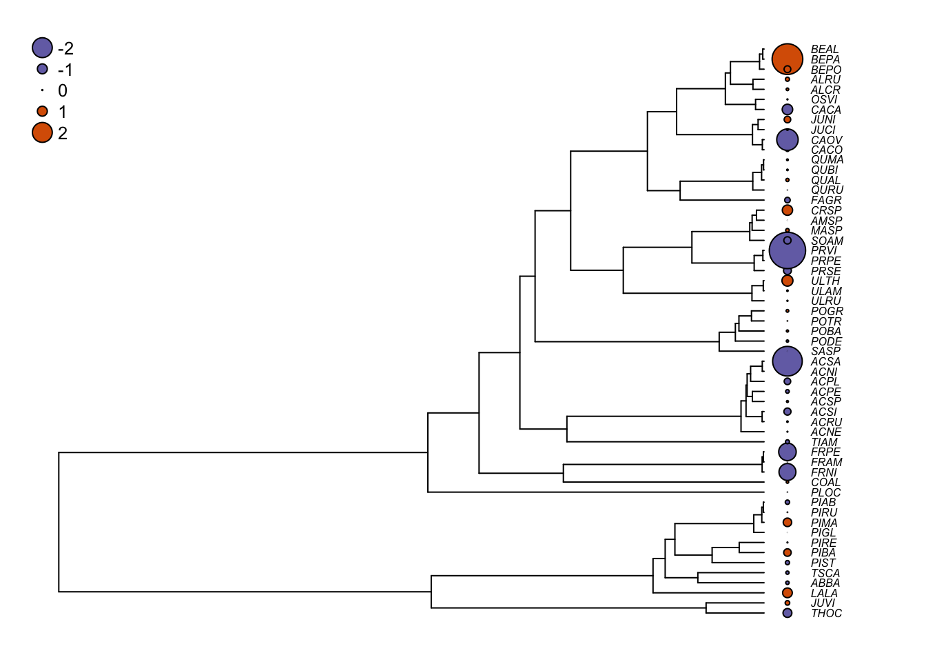
If you compare with the ordinary least squares optimization, the residuals are much less phylogenetically correlated.
5.3.1 Other correlation structures
In the previous PGLS, we have used the corSymm structure to pass the phylogenetic correlation structure to the gls. This is perfectly fine, but there are more simple ways. Julien Dutheil has developped phylogenetic structures to be used especially in PGLS.
The one we used above is equivalent to the corBrownian structure of ape. This approach is easier and you just have to pass the tree to the correlation structure. Here is the same example using the corBrownian structure.
# Get the correlation structure
bm.corr <- corBrownian(phy=seedplantstree, form=~Code)
# PGLS
shade.pgls1b <- gls(Shade ~ Wd, data = seedplantsdata, correlation=bm.corr)
summary(shade.pgls1b)
## Generalized least squares fit by REML
## Model: Shade ~ Wd
## Data: seedplantsdata
## AIC BIC logLik
## 214.3762 220.3982 -104.1881
##
## Correlation Structure: corBrownian
## Formula: ~Code
## Parameter estimate(s):
## numeric(0)
##
## Coefficients:
## Value Std.Error t-value p-value
## (Intercept) 0.911433 4.409058 0.2067184 0.8370
## Wd 4.361028 1.693349 2.5753865 0.0127
##
## Correlation:
## (Intr)
## Wd -0.166
##
## Standardized residuals:
## Min Q1 Med Q3 Max
## -0.26890642 -0.16431866 -0.02645422 0.09638984 0.34953444
##
## Residual standard error: 7.455109
## Degrees of freedom: 57 total; 55 residualYou can see that the results are identical. The only difference is that the correlation structure is not outputed in the summary. The numeric(0) means that no parameter was estimated during the optimization (it is fixed).
Now, you might wonder why the correlation structure is called corBrownian. This is because is uses Brownian motion to model the evolution along the branch of the tree. This is often refferred as a neutral model. If you want to know more about the Brownian Motion model, you can look at the section 12 on this model.